p.21

Covariance Derivation

The covariance between two random variables $X_1$ and $X_2$ is defined as:

\text{Cov}(X_1, X_2) = \mathbb{E}\left[(X_1 - \mathbb{E}(X_1))(X_2 - \mathbb{E}(X_2))\right]

Step 1: Expanding the expression

First, expand the product inside the expectation:

(X_1 - \mathbb{E}(X_1))(X_2 - \mathbb{E}(X_2)) = X_1X_2 - X_1\mathbb{E}(X_2) - \mathbb{E}(X_1)X_2 + \mathbb{E}(X_1)\mathbb{E}(X_2)

Step 2: Taking the expectation

Now, take the expectation of both sides:

\mathbb{E}\left[(X_1 - \mathbb{E}(X_1))(X_2 - \mathbb{E}(X_2))\right] = \mathbb{E}(X_1X_2) - \mathbb{E}(X_1)\mathbb{E}(X_2) - \mathbb{E}(X_1)\mathbb{E}(X_2) + \mathbb{E}(X_1)\mathbb{E}(X_2)

Step 3: Simplifying the result

Notice that the terms $\mathbb{E}(X_1)\mathbb{E}(X_2)$ cancel out:

\mathbb{E}(X_1X_2) - \mathbb{E}(X_1)\mathbb{E}(X_2)

Thus, we arrive at the final formula for the covariance:

\text{Cov}(X_1, X_2) = \mathbb{E}(X_1X_2) - \mathbb{E}(X_1)\mathbb{E}(X_2)

p.22

Covariance Derivation in Confirmatory Factor Analysis

We start with the observed variables $x_1$ and $x_2$ :

x_1 = \lambda_1 \xi_1 + \delta_1

x_2 = \lambda_2 \xi_1 + \delta_2

We want to find $\text{Cov}(x_1, x_2)$ :

\text{Cov}(x_1, x_2) = \text{Cov}(\lambda_1 \xi_1 + \delta_1, \lambda_2 \xi_1 + \delta_2)

Using bilinearity of covariance:

= \lambda_1 \lambda_2 \text{Cov}(\xi_1, \xi_1) + \lambda_1 \text{Cov}(\xi_1, \delta_2) + \lambda_2 \text{Cov}(\delta_1, \xi_1) + \text{Cov}(\delta_1, \delta_2)

Assuming:

$\text{Cov}(\xi_1, \delta_2) = 0$
$\text{Cov}(\delta_1, \xi_1) = 0$
$\text{Cov}(\delta_1, \delta_2) = 0$
$\text{Var}(\xi_1) = \phi_{11}$

Then:

\text{Cov}(x_1, x_2) = \lambda_1 \lambda_2 \phi_{11}

p.23

1. Derivation: Cov(x, c′) = 0

Let $\mathbf{x}$ be a random vector and $\mathbf{c}$ a constant vector.

\text{Cov}(\mathbf{x}, \mathbf{c}^\top) = \mathbb{E} \left[ (\mathbf{x} - \mathbb{E}[\mathbf{x}])(\mathbf{c}^\top - \mathbb{E}[\mathbf{c}^\top]) \right]

But since $\mathbf{c}^\top$ is constant, $\mathbb{E}[\mathbf{c}^\top] = \mathbf{c}^\top$ , so:

\mathbf{c}^\top - \mathbb{E}[\mathbf{c}^\top] = \mathbf{0}

Hence:

\text{Cov}(\mathbf{x}, \mathbf{c}^\top) = \mathbb{E} \left[ (\mathbf{x} - \mathbb{E}[\mathbf{x}]) \cdot \mathbf{0} \right] = \mathbf{0}

2. Derivation: Var(x) = Cov(x, x′) = Σ

By definition:

\text{Var}(\mathbf{x}) = \text{Cov}(\mathbf{x}, \mathbf{x}^\top) = \mathbb{E} \left[ (\mathbf{x} - \mathbb{E}[\mathbf{x}])(\mathbf{x} - \mathbb{E}[\mathbf{x}])^\top \right]

This is the population covariance matrix, denoted as:

\boldsymbol{\Sigma}

3. Numerical Example in R

# Set seed and generate data
set.seed(123)

# Simulate random vector x (5 observations, 3 variables)
x <- matrix(c(1, 2, 3, 4, 5,
              2, 3, 4, 5, 6,
              5, 4, 3, 2, 1), ncol = 3)

x

##      [,1] [,2] [,3]
## [1,]    1    2    5
## [2,]    2    3    4
## [3,]    3    4    3
## [4,]    4    5    2
## [5,]    5    6    1

x_centered <- scale(x, center = TRUE, scale = FALSE)
x_centered

##      [,1] [,2] [,3]
## [1,]   -2   -2    2
## [2,]   -1   -1    1
## [3,]    0    0    0
## [4,]    1    1   -1
## [5,]    2    2   -2
## attr(,"scaled:center")
## [1] 3 4 3

4. Confirm Var(x) = Cov(x, x′)

# Compute covariance matrix of x manually
# population covariance matrix
Sigma_manual_p <- t(x_centered) %*% x_centered / (nrow(x))
Sigma_manual_p

##      [,1] [,2] [,3]
## [1,]    2    2   -2
## [2,]    2    2   -2
## [3,]   -2   -2    2

# sample covariance matrix
Sigma_manual_s <- t(x_centered) %*% x_centered / (nrow(x) - 1)
Sigma_manual_s

##      [,1] [,2] [,3]
## [1,]  2.5  2.5 -2.5
## [2,]  2.5  2.5 -2.5
## [3,] -2.5 -2.5  2.5

# Compare with built-in cov()
# sample covariance matrix
Sigma_builtin <- cov(x)
Sigma_builtin

##      [,1] [,2] [,3]
## [1,]  2.5  2.5 -2.5
## [2,]  2.5  2.5 -2.5
## [3,] -2.5 -2.5  2.5

p.28

Step 1: Create the data for Disposable Income and Consumers’ Expenditures

income <- c(433, 483, 479, 486, 494, 498, 511, 534, 478, 440, 372, 381, 419, 449, 511, 520, 477, 517, 548, 629)

consum <- c(394, 423, 437, 434, 447, 447, 466, 474, 439, 399, 350, 364, 392, 416, 463, 469, 444, 471, 494, 529)

Step 2: Combine the data into a matrix

data <- cbind(consum, income)

data

##       consum income
##  [1,]    394    433
##  [2,]    423    483
##  [3,]    437    479
##  [4,]    434    486
##  [5,]    447    494
##  [6,]    447    498
##  [7,]    466    511
##  [8,]    474    534
##  [9,]    439    478
## [10,]    399    440
## [11,]    350    372
## [12,]    364    381
## [13,]    392    419
## [14,]    416    449
## [15,]    463    511
## [16,]    469    520
## [17,]    444    477
## [18,]    471    517
## [19,]    494    548
## [20,]    529    629

Step 3: Center the data by subtracting the mean of each variable

Z <- scale(data, center = TRUE, scale = FALSE)  # Centers the data (but doesn't scale it)
Z

##       consum  income
##  [1,]  -43.6  -49.95
##  [2,]  -14.6    0.05
##  [3,]   -0.6   -3.95
##  [4,]   -3.6    3.05
##  [5,]    9.4   11.05
##  [6,]    9.4   15.05
##  [7,]   28.4   28.05
##  [8,]   36.4   51.05
##  [9,]    1.4   -4.95
## [10,]  -38.6  -42.95
## [11,]  -87.6 -110.95
## [12,]  -73.6 -101.95
## [13,]  -45.6  -63.95
## [14,]  -21.6  -33.95
## [15,]   25.4   28.05
## [16,]   31.4   37.05
## [17,]    6.4   -5.95
## [18,]   33.4   34.05
## [19,]   56.4   65.05
## [20,]   91.4  146.05
## attr(,"scaled:center")
## consum income 
## 437.60 482.95

Step 4: Compute Z’ (transpose of Z)

Z_t <- t(Z)
Z_t

##          [,1]   [,2]  [,3]  [,4]  [,5]  [,6]  [,7]  [,8]  [,9]  [,10]   [,11]
## consum -43.60 -14.60 -0.60 -3.60  9.40  9.40 28.40 36.40  1.40 -38.60  -87.60
## income -49.95   0.05 -3.95  3.05 11.05 15.05 28.05 51.05 -4.95 -42.95 -110.95
##          [,12]  [,13]  [,14] [,15] [,16] [,17] [,18] [,19]  [,20]
## consum  -73.60 -45.60 -21.60 25.40 31.40  6.40 33.40 56.40  91.40
## income -101.95 -63.95 -33.95 28.05 37.05 -5.95 34.05 65.05 146.05
## attr(,"scaled:center")
## consum income 
## 437.60 482.95

Step 5: Compute Z’Z (matrix multiplication of Z’ and Z)

Z_t_Z <- Z_t %*% Z
Z_t_Z

##         consum   income
## consum 35886.8 47584.60
## income 47584.6 64992.95

Step 6: Apply the 1/(N-1) factor

N <- nrow(Z)  # Number of observations (rows)
cov_matrix_manual <- (1 / (N - 1)) * Z_t_Z

# Display the result
print(cov_matrix_manual)

##          consum   income
## consum 1888.779 2504.453
## income 2504.453 3420.682

p.28

Introduction

In multivariate statistics, it is often important to detect observations that deviate significantly from the center of the multivariate data cloud. One useful tool is the matrix:

\mathbf{A} = \mathbf{Z(Z'Z)^{-1}Z'}

Where:

$\mathbf{Z}$ is the mean-centered data matrix of size $N \times (p + q)$ ,

$\mathbf{Z}'\mathbf{Z}$ is the cross-product matrix,

$(\mathbf{Z}'\mathbf{Z})^{-1}$ is its inverse,

$\mathbf{A}$ is a square $N \times N$ matrix whose diagonal entries $a_{ii}$ represent the multivariate “distance” of each observation from the center.

The average value of $a_{ii}$ is:

\frac{(p + q)}{N}

Observations with much higher $a_{ii}$ values than the average are potential multivariate outliers.

Step-by-Step Example

We will use a simple example dataset with 3 observations and 2 variables.

# Define the data matrix (3 observations, 2 variables)
X <- matrix(c(2, 3, 4, 4, 6, 5), ncol = 2, byrow = FALSE)
colnames(X) <- c("X1", "X2")
rownames(X) <- paste0("Obs", 1:3)
X

##      X1 X2
## Obs1  2  4
## Obs2  3  6
## Obs3  4  5

Step 1: Center the Data (Create Z)

We subtract the mean from each variable to obtain the matrix $\mathbf{Z}$ .

Z <- scale(X, center = TRUE, scale = FALSE)
Z

##      X1 X2
## Obs1 -1 -1
## Obs2  0  1
## Obs3  1  0
## attr(,"scaled:center")
## X1 X2 
##  3  5

Step 2: Compute $\mathbf{Z}'\mathbf{Z}$

ZtZ <- t(Z) %*% Z
ZtZ

##    X1 X2
## X1  2  1
## X2  1  2

Step 3: Compute $(\mathbf{Z}'\mathbf{Z})^{-1}$

ZtZ_inv <- solve(ZtZ)
ZtZ_inv

##            X1         X2
## X1  0.6666667 -0.3333333
## X2 -0.3333333  0.6666667

Step 4: Compute $\mathbf{A} = \mathbf{Z}(\mathbf{Z}'\mathbf{Z})^{-1}\mathbf{Z}'$

A <- Z %*% ZtZ_inv %*% t(Z)
round(A, 3)

##        Obs1   Obs2   Obs3
## Obs1  0.667 -0.333 -0.333
## Obs2 -0.333  0.667 -0.333
## Obs3 -0.333 -0.333  0.667

Step 5: Extract Diagonal Elements $a_{ii}$

These diagonal values represent the multivariate distance for each observation.

a_ii <- diag(A)
names(a_ii) <- rownames(X)
a_ii

##      Obs1      Obs2      Obs3 
## 0.6666667 0.6666667 0.6666667

Step 6: Compare to Expected Average

p_plus_q <- ncol(Z)  # total number of observed variables (p + q)
N <- nrow(Z)  # number of observations
expected_mean <- p_plus_q / N
expected_mean

## [1] 0.6666667

Any $a_{ii}$ significantly greater than 0.6666667 may indicate a multivariate outlier.

Step 7: Visualization

barplot(a_ii, names.arg = names(a_ii), 
        main = "Multivariate Distance (a_ii) for Each Observation", 
        ylab = "a_ii", col = "skyblue", ylim = c(0, 1))
abline(h = expected_mean, col = "red", lty = 2)
legend("topright", legend = paste("Expected Mean =", round(expected_mean, 3)), 
       col = "red", lty = 2)

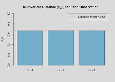
Conclusion

Matrix $\mathbf{A} = \mathbf{Z(Z'Z)^{-1}Z'}$ provides a way to measure the multivariate distance of each observation.
Diagonal values $a_{ii}$ indicate how far each case is from the multivariate mean.
The average of the $a_{ii}$ ’s is $\frac{(p + q)}{N}$ , which provides a benchmark.
Observations with high $a_{ii}$ values are flagged as potential outliers in multivariate space.

This method is especially helpful in the context of SEM, factor analysis, or other multivariate procedures where unusual cases may affect model fit or estimates.

p. 30

Introduction

The formula for calculating multidimensional outliers:

Z(Z'Z)^{-1}Z'

Where:

$Z$ is the standardized data matrix.

$Z'Z$ is the product of the transposed $Z$ matrix and $Z$ itself.

$(Z'Z)^{-1}$ is the inverse of the matrix $Z'Z$ .

The final result gives a measure of how far each observation is from the multivariate centroid.

We will apply this formula to a dataset that contains estimates of cloud cover (COVER1, COVER2, COVER3).

Data Preparation

# Define the data
data <- data.frame(
  COVER1 = c(0, 20, 80, 50, 5, 1, 5, 0, 10, 0, 0, 10, 0, 10, 0, 0, 5, 10, 20, 35, 90, 50, 35, 25, 0, 0, 10, 40, 35, 55, 35, 0, 0, 5, 20, 0, 0, 0, 15, 95, 40, 40, 15, 30, 75, 100, 100, 100, 100, 100, 100, 100, 0, 5, 80, 80, 80, 40, 20, 1),
  COVER2 = c(5, 20, 85, 50, 2, 1, 5, 0, 15, 0, 0, 30, 2, 10, 0, 0, 0, 20, 45, 75, 99, 90, 85, 15, 0, 0, 10, 75, 70, 90, 95, 0, 0, 1, 60, 0, 0, 0, 55, 0, 35, 50, 60, 30, 85, 100, 90, 95, 95, 99, 30, 5, 0, 5, 90, 95, 90, 55, 40, 0),
  COVER3 = c(0, 20, 90, 70, 5, 2, 2, 0, 5, 0, 0, 10, 2, 5, 0, 0, 20, 20, 15, 60, 100, 80, 70, 40, 0, 0, 20, 30, 20, 90, 80, 0, 0, 2, 50, 0, 0, 0, 50, 40, 30, 40, 5, 15, 75, 100, 85, 100, 100, 100, 95, 95, 0, 5, 85, 80, 70, 50, 5, 0)
)

dplyr::glimpse(data)

## Rows: 60
## Columns: 3
## $ COVER1 <dbl> 0, 20, 80, 50, 5, 1, 5, 0, 10, 0, 0, 10, 0, 10, 0, 0, 5, 10, 20…
## $ COVER2 <dbl> 5, 20, 85, 50, 2, 1, 5, 0, 15, 0, 0, 30, 2, 10, 0, 0, 0, 20, 45…
## $ COVER3 <dbl> 0, 20, 90, 70, 5, 2, 2, 0, 5, 0, 0, 10, 2, 5, 0, 0, 20, 20, 15,…

# View the data to check it
head(data)

##   COVER1 COVER2 COVER3
## 1      0      5      0
## 2     20     20     20
## 3     80     85     90
## 4     50     50     70
## 5      5      2      5
## 6      1      1      2

Mean-Centering

We will now mean-center the data to create the Z matrix.

# Mean-centering the data (subtracting the mean of each column from the data)
Z <- scale(data, center = TRUE, scale = FALSE)

Z

##       COVER1 COVER2 COVER3
##  [1,] -32.95 -32.65 -35.55
##  [2,] -12.95 -17.65 -15.55
##  [3,]  47.05  47.35  54.45
##  [4,]  17.05  12.35  34.45
##  [5,] -27.95 -35.65 -30.55
##  [6,] -31.95 -36.65 -33.55
##  [7,] -27.95 -32.65 -33.55
##  [8,] -32.95 -37.65 -35.55
##  [9,] -22.95 -22.65 -30.55
## [10,] -32.95 -37.65 -35.55
## [11,] -32.95 -37.65 -35.55
## [12,] -22.95  -7.65 -25.55
## [13,] -32.95 -35.65 -33.55
## [14,] -22.95 -27.65 -30.55
## [15,] -32.95 -37.65 -35.55
## [16,] -32.95 -37.65 -35.55
## [17,] -27.95 -37.65 -15.55
## [18,] -22.95 -17.65 -15.55
## [19,] -12.95   7.35 -20.55
## [20,]   2.05  37.35  24.45
## [21,]  57.05  61.35  64.45
## [22,]  17.05  52.35  44.45
## [23,]   2.05  47.35  34.45
## [24,]  -7.95 -22.65   4.45
## [25,] -32.95 -37.65 -35.55
## [26,] -32.95 -37.65 -35.55
## [27,] -22.95 -27.65 -15.55
## [28,]   7.05  37.35  -5.55
## [29,]   2.05  32.35 -15.55
## [30,]  22.05  52.35  54.45
## [31,]   2.05  57.35  44.45
## [32,] -32.95 -37.65 -35.55
## [33,] -32.95 -37.65 -35.55
## [34,] -27.95 -36.65 -33.55
## [35,] -12.95  22.35  14.45
## [36,] -32.95 -37.65 -35.55
## [37,] -32.95 -37.65 -35.55
## [38,] -32.95 -37.65 -35.55
## [39,] -17.95  17.35  14.45
## [40,]  62.05 -37.65   4.45
## [41,]   7.05  -2.65  -5.55
## [42,]   7.05  12.35   4.45
## [43,] -17.95  22.35 -30.55
## [44,]  -2.95  -7.65 -20.55
## [45,]  42.05  47.35  39.45
## [46,]  67.05  62.35  64.45
## [47,]  67.05  52.35  49.45
## [48,]  67.05  57.35  64.45
## [49,]  67.05  57.35  64.45
## [50,]  67.05  61.35  64.45
## [51,]  67.05  -7.65  59.45
## [52,]  67.05 -32.65  59.45
## [53,] -32.95 -37.65 -35.55
## [54,] -27.95 -32.65 -30.55
## [55,]  47.05  52.35  49.45
## [56,]  47.05  57.35  44.45
## [57,]  47.05  52.35  34.45
## [58,]   7.05  17.35  14.45
## [59,] -12.95   2.35 -30.55
## [60,] -31.95 -37.65 -35.55
## attr(,"scaled:center")
## COVER1 COVER2 COVER3 
##  32.95  37.65  35.55

# Check the mean-centered data (Z matrix)
head(Z)

##      COVER1 COVER2 COVER3
## [1,] -32.95 -32.65 -35.55
## [2,] -12.95 -17.65 -15.55
## [3,]  47.05  47.35  54.45
## [4,]  17.05  12.35  34.45
## [5,] -27.95 -35.65 -30.55
## [6,] -31.95 -36.65 -33.55

Calculating $Z'Z$

Next, we compute the product of the transposed matrix $Z$ and the matrix $Z$ .

# Calculate Z'Z (transposed Z matrix multiplied by Z)
ZZT <- t(Z) %*% Z

# View the result of Z'Z
ZZT

##          COVER1   COVER2   COVER3
## COVER1 76734.85 60191.95 72989.65
## COVER2 60191.95 86335.65 70795.55
## COVER3 72989.65 70795.55 82812.85

Inverse of $Z'Z$

Now, we calculate the inverse of the matrix $Z'Z$ .

# Calculate the inverse of Z'Z
ZZT_inv <- solve(ZZT)

# View the inverse of Z'Z
ZZT_inv

##               COVER1        COVER2        COVER3
## COVER1  8.186873e-05  6.996057e-06 -7.813835e-05
## COVER2  6.996057e-06  3.933723e-05 -3.979504e-05
## COVER3 -7.813835e-05 -3.979504e-05  1.149653e-04

Calculate $Z(Z'Z)^{-1}Z'$

Finally, using the inverse of $Z'Z$ , we compute the multidimensional outlier scores.

# Calculate the multidimensional outliers
outliers <- Z %*% ZZT_inv %*% t(Z)

# Extract the diagonal of the outlier matrix (outlier scores)
outlier_scores <- diag(outliers)

# View the outlier scores for each observation
outlier_scores

##  [1] 0.015726795 0.003667134 0.035888471 0.043531791 0.015067469 0.016818904
##  [7] 0.014336636 0.017711895 0.013230015 0.017711895 0.017711895 0.015735922
## [13] 0.016767037 0.012571539 0.017711895 0.017711895 0.047722524 0.011226588
## [19] 0.033505745 0.044503013 0.051723149 0.067601060 0.085473686 0.043702080
## [25] 0.017711895 0.017711895 0.019881286 0.088784132 0.115257068 0.090112579
## [31] 0.141386847 0.017711895 0.017711895 0.016124246 0.056874143 0.017711895
## [37] 0.017711895 0.017711895 0.078447969 0.310744264 0.012569282 0.004286889
## [43] 0.116357798 0.029894426 0.031821437 0.061860674 0.081910183 0.059274389
## [49] 0.059274389 0.061186068 0.182763526 0.317232262 0.017711895 0.013128462
## [55] 0.034993660 0.045793479 0.063100245 0.005752862 0.064705791 0.017427449

sum(outlier_scores)

## [1] 3

Sample Covariance Matrix

Z_t <- t(Z)
Z_t

##          [,1]   [,2]  [,3]  [,4]   [,5]   [,6]   [,7]   [,8]   [,9]  [,10]
## COVER1 -32.95 -12.95 47.05 17.05 -27.95 -31.95 -27.95 -32.95 -22.95 -32.95
## COVER2 -32.65 -17.65 47.35 12.35 -35.65 -36.65 -32.65 -37.65 -22.65 -37.65
## COVER3 -35.55 -15.55 54.45 34.45 -30.55 -33.55 -33.55 -35.55 -30.55 -35.55
##         [,11]  [,12]  [,13]  [,14]  [,15]  [,16]  [,17]  [,18]  [,19] [,20]
## COVER1 -32.95 -22.95 -32.95 -22.95 -32.95 -32.95 -27.95 -22.95 -12.95  2.05
## COVER2 -37.65  -7.65 -35.65 -27.65 -37.65 -37.65 -37.65 -17.65   7.35 37.35
## COVER3 -35.55 -25.55 -33.55 -30.55 -35.55 -35.55 -15.55 -15.55 -20.55 24.45
##        [,21] [,22] [,23]  [,24]  [,25]  [,26]  [,27] [,28]  [,29] [,30] [,31]
## COVER1 57.05 17.05  2.05  -7.95 -32.95 -32.95 -22.95  7.05   2.05 22.05  2.05
## COVER2 61.35 52.35 47.35 -22.65 -37.65 -37.65 -27.65 37.35  32.35 52.35 57.35
## COVER3 64.45 44.45 34.45   4.45 -35.55 -35.55 -15.55 -5.55 -15.55 54.45 44.45
##         [,32]  [,33]  [,34]  [,35]  [,36]  [,37]  [,38]  [,39]  [,40] [,41]
## COVER1 -32.95 -32.95 -27.95 -12.95 -32.95 -32.95 -32.95 -17.95  62.05  7.05
## COVER2 -37.65 -37.65 -36.65  22.35 -37.65 -37.65 -37.65  17.35 -37.65 -2.65
## COVER3 -35.55 -35.55 -33.55  14.45 -35.55 -35.55 -35.55  14.45   4.45 -5.55
##        [,42]  [,43]  [,44] [,45] [,46] [,47] [,48] [,49] [,50] [,51]  [,52]
## COVER1  7.05 -17.95  -2.95 42.05 67.05 67.05 67.05 67.05 67.05 67.05  67.05
## COVER2 12.35  22.35  -7.65 47.35 62.35 52.35 57.35 57.35 61.35 -7.65 -32.65
## COVER3  4.45 -30.55 -20.55 39.45 64.45 49.45 64.45 64.45 64.45 59.45  59.45
##         [,53]  [,54] [,55] [,56] [,57] [,58]  [,59]  [,60]
## COVER1 -32.95 -27.95 47.05 47.05 47.05  7.05 -12.95 -31.95
## COVER2 -37.65 -32.65 52.35 57.35 52.35 17.35   2.35 -37.65
## COVER3 -35.55 -30.55 49.45 44.45 34.45 14.45 -30.55 -35.55
## attr(,"scaled:center")
## COVER1 COVER2 COVER3 
##  32.95  37.65  35.55

Z_t_Z <- Z_t %*% Z
Z_t_Z

##          COVER1   COVER2   COVER3
## COVER1 76734.85 60191.95 72989.65
## COVER2 60191.95 86335.65 70795.55
## COVER3 72989.65 70795.55 82812.85

N <- nrow(Z)  # Number of observations (rows)
cov_matrix_manual <- (1 / (N - 1)) * Z_t_Z

# Display the result
print(cov_matrix_manual)

##          COVER1   COVER2   COVER3
## COVER1 1300.591 1020.203 1237.113
## COVER2 1020.203 1463.316 1199.925
## COVER3 1237.113 1199.925 1403.608

SEM (notes for myself)

p.21

Covariance Derivation

Step 1: Expanding the expression

Step 2: Taking the expectation

Step 3: Simplifying the result

p.22

Covariance Derivation in Confirmatory Factor Analysis

p.23

1. Derivation: Cov(x, c′) = 0

2. Derivation: Var(x) = Cov(x, x′) = Σ

3. Numerical Example in R

4. Confirm Var(x) = Cov(x, x′)

p.28

Step 1: Create the data for Disposable Income and Consumers’ Expenditures

Step 2: Combine the data into a matrix

Step 3: Center the data by subtracting the mean of each variable

Step 4: Compute Z’ (transpose of Z)

Step 5: Compute Z’Z (matrix multiplication of Z’ and Z)

Step 6: Apply the 1/(N-1) factor

p.28

Introduction

Step-by-Step Example

Step 1: Center the Data (Create Z)

Step 2: Compute Z′Z\mathbf{Z}'\mathbf{Z}Z′Z

Step 3: Compute (Z′Z)−1(\mathbf{Z}'\mathbf{Z})^{-1}(Z′Z)−1

Step 4: Compute A=Z(Z′Z)−1Z′\mathbf{A} = \mathbf{Z}(\mathbf{Z}'\mathbf{Z})^{-1}\mathbf{Z}'A=Z(Z′Z)−1Z′

Step 5: Extract Diagonal Elements aiia_{ii}aii​

Step 6: Compare to Expected Average

Step 7: Visualization

Conclusion

p. 30

Introduction

Data Preparation

Mean-Centering

Calculating Z′ZZ'ZZ′Z

Inverse of Z′ZZ'ZZ′Z

Calculate Z(Z′Z)−1Z′Z(Z'Z)^{-1}Z'Z(Z′Z)−1Z′

Sample Covariance Matrix

Step 2: Compute $\mathbf{Z}'\mathbf{Z}$

Step 3: Compute $(\mathbf{Z}'\mathbf{Z})^{-1}$

Step 4: Compute $\mathbf{A} = \mathbf{Z}(\mathbf{Z}'\mathbf{Z})^{-1}\mathbf{Z}'$

Step 5: Extract Diagonal Elements $a_{ii}$

Calculating $Z'Z$

Inverse of $Z'Z$

Calculate $Z(Z'Z)^{-1}Z'$